1 Genomics
Introduction
Leaving Certificate Syllabus
This chapter complements:
- Biology section 2.5 Genetics.
The Structure of DNA
 Deoxyribonucleic acid (DNA) is made up of two strands which wind around each other to form a structure called the double helix. Each strand has a backbone made up of alternative sugar (deoxyribose) and phosphate groups. Attached to each sugar is one of four nucleotide bases; A (Adenine), C (Cytosine), G (Guanine) and T (Thymine). These bases are chemically ‘complimentary’ to each other – A is complementary to T and C is complementary to G. There are approximately 3 billion base pairs in the human genome!
Each series of 3 DNA bases is called a ‘codon’, encoding one of 20 amino acids. For example, the codon ATG encodes the amino acid ‘methionine’. Amino acids form a contiguous chain of polymers that folds into a specific structure yielding a biologically functional protein.
Genes Specify Proteins
Within the vast stretches of DNA in our genome are biologically functional stretches of DNA called genes.
Each gene provides instructions for a functional product, that is, a molecule needed to perform a job in the cell. In many cases, the functional product of a gene is a protein.
What does a gene look like?
Exercise – Visualising the human genome
To help you visualise these functional regions of the human genome, we will use an application called the Integrative Genomics Viewer (IGV) which is a high-performance, easy-to-use, interactive tool for the visual exploration of genomic data. Once we have selected the genome to view, an annotation track is automatically loaded in the browser (you may have to zoom in to view it).
The annotation track marks the start and end coordinates of (known) genes in our DNA. The vast majority of functional products listed in the annotation tracks are proteins, which is the main job of genes – to produce proteins. Such genes are known as protein-coding genes.
1. Navigate to the IGV application using a web browser: https://igv.org/app/
2. Select the ‘Genome‘ tab and select ‘Human (GRCh38/hg38)’ which is the most current version of the human genome.
3. In the search bar, you can enter the specific coordinates of a gene, or the gene name. Enter ‘PTEN‘ to view the PTEN gene which is located at chr10:87,862,624-87,972,930.
4. You will notice that there are two blue lines representing PTEN. These are two isoforms of the PTEN gene. This means that the PTEN gene can produce two proteins of similar function – but they will differ slightly in composition.
5. Google the PTEN gene – you will discover it is a very important gene in our genome!
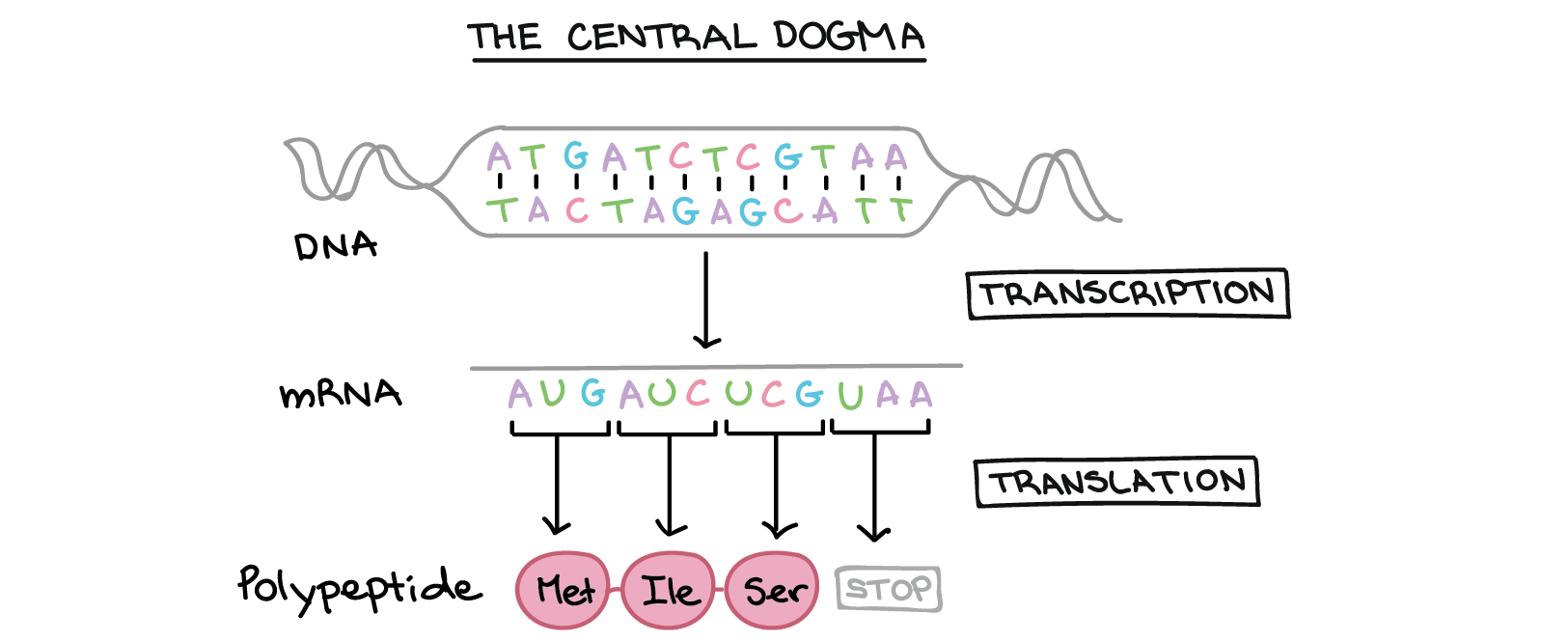
The Central Dogma
- Transcription: the DNA sequence of a gene is copied to make a mRNA molecule. This step is called transcription because it involves rewriting, or transcribing, the DNA sequence in a similar RNA “alphabet”.
- Translation: the sequence of the mRNA is decoded to produce a contiguous chain of amino acids. The name translation refers to the nucleotide sequence of the mRNA sequence being translated into a completely different “language” of amino acids.
The process of activating a gene to produce a functional protein is known as gene expression.
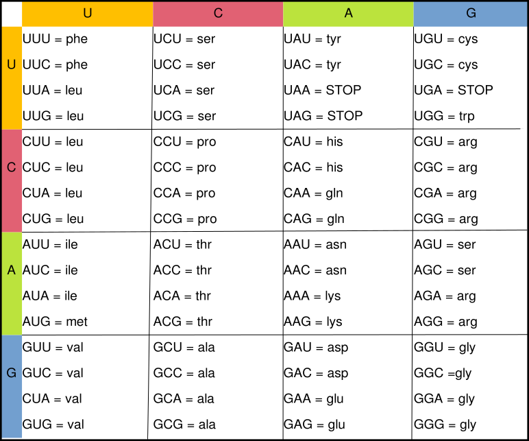
Codon Chart
The amino acids encoded by each of the RNA codons are outlined in the table below:

QUIZ!
Answer the questions corresponding to images 1, 2 and 3.
RNA-Sequencing
A popular experiment in genomics is called RNA-Sequencing where the messenger RNA in a cell is captured and counted using high throughput sequencing technologies and computational algorithms. This allows researchers to quantify the expression of all genes in our genome – seeing what genes are turned on or off, and by how much each gene is expressed. It can be useful to use RNA-Sequencing to compare normal cells vs. disease cells to identify genes that have been irreparably broken.

- Library preparation.
- Sequencing.
- Data Analysis (that’s us!).
1. Library Preparation
Library preparation involves capturing the RNA in cells and preparing the sample for sequencing. It can be divided into 6 steps:
- Cells are burst open, RNA is isolated and DNA is removed.
- We need to cut the RNA into smaller fragments – the sequencing machine can only handle sizes of 200-300 nucleotides.
- The fragmented RNA is converted to DNA (DNA is more stable than RNA, and we do not lose any information).
- Sequencing adapters (human-designed sequences) are added to the newly synthesized DNA.
- PCR is used to make millions of copies of the fragmented sequences.
- The sample is checked – are the lengths of the amplified fragments ok? (200-300nt) and do we have enough RNA for the experiment?

2. Sequencing
The samples containing the captured RNA are then sent to a laboratory where sequencing is performed. Below is a broad schematic of how sequencing works:
- In the top figure, the PCR fragments are bound to the flow cell using their adapter sequences. The flow cell contains millions of complimentary adapter sequences to capture the PCR fragments for sequencing.
- DNA bases (A, T, G, C) are added to the flow cells, where they will bind to their complementary base. These DNA bases are special in that they have a unique flourescent probe attached to them prior to adding them to the flow cell.
- A laser is used to excite the fluorescent probes attached to the newly added DNA molecules, emitting blue (adenosine), yellow (cytosine), red (thymine) and green (guanine) light for each base. This light is captured by imaging, whereby computer software notes which base was synthesized at each position.
- In the bottom figure, the probes are washed away and the process is repeated for 100-150 cycles.

FASTQ Files
FASTQ files are used to store the output from sequencing machines. See below for the first 4 sequences stored in a FASTQ file (each sequence has 4 lines of information):
@SRR6357073.31043222 31043222/1 kraken:taxid|4932
GTTTTCGATTTCGAATTATTTGTTTTTTGAGGATTCCGAGCTATAACTTTGGGTTTGGTTGTATTCGTATAGCTGCGAGAATCATTCTTCTCATCACTCGG
+
BBBBBFFFFFFFF/FFFFFFFFFFFFFFFFFFFFFFFFFFFFFFFFFFFFFFFFF<<FFFFFFFFFFFFFFFFFFFFFFFFFFFFFFFFFFFFFFFFFFFF
@SRR6357073.8331722 8331722/1 kraken:taxid|4932
ATTGGATTGCATGCCTGAGTCGTAAGTGTCAGGATGCTGAATATCACCTCTTGCAACAAATCTAGCTTTATGAGTACCGTCACGTTTCTTGTTGAAGAGAT
+
<BBBBFB/FF<B/<BB//B/</<<FFFFFFB/B</<F<FFFFFBF<BFFFB<F<FBFB<BFBBB</FF/FFFFFF/<FBFFFFF<FFFBFFFFBFBBB/FB
@SRR6357073.7254397 7254397/1 kraken:taxid|4932
CTTGCAACAAATCTAGCTTTATGAGTACCGTCACGGTTCTTGTTGAAGATAAACATTGAGTTTATTACTCTTTTAGGGTCTATTTCTGTTCTGTCATAATA
+
BBBB<FFFFFFF<FFFFFF<FFFBF/B/FFFFBFF///<FFFFFFBFF<FFFFFFFFB//</FBFFF<BFFFFFFFFFFFFFFFFF//B<FBFFF<<<F//
@SRR6357073.19215418 19215418/1 kraken:taxid|4932
ATTTTACAGGGCGATCGCTAAGCTTAATCAACTTCTTCGACAGTTGGACCTTCAGCTTCTGGAGCTGGAGGAGCACCACCTGGGAAACCACCTGGAGCTGC
+
BBBBBFFFFFFFFFFFFFFFFFFFFFFFFFFFFFFFFFFFFFFFFFFFFFFFFFBFFFFFFFFFFFFFFFFFFFFFFFFFFFFFFFFFFFFFFFFFFFFFF
- Line 1 always begins with a @ indicating the sequencing run (google SRR6357073 to find out more about the origin of this run), sequencing machine and cluster information.
- Line 2 is the cDNA sequence that was derived from the original RNA template.
- Line 3 is always a + – probably used as a separator.
- Line 4 is the base quality scores represented by ‘ASCII characters’, i.e how confident the machine was in calling each base. See the figure below for the probability scores (of an incorrectly called base) associated with each ASCII character.

In the example FASTQ file, the first sequence starts with ‘GT’ (guanine, thymine) which has the corresponding ASCII characters ‘BB’. By checking the table above, we can see that B means the probability of error of the call is 0.00050 – or a 1 in 2000 chance of being incorrect. Even with such great odds, sequencing is not perfect due to the sheer size of our genome, PCR amplification and the 150 cycles run; we are likely to come across 1 in 2000 errors several times!
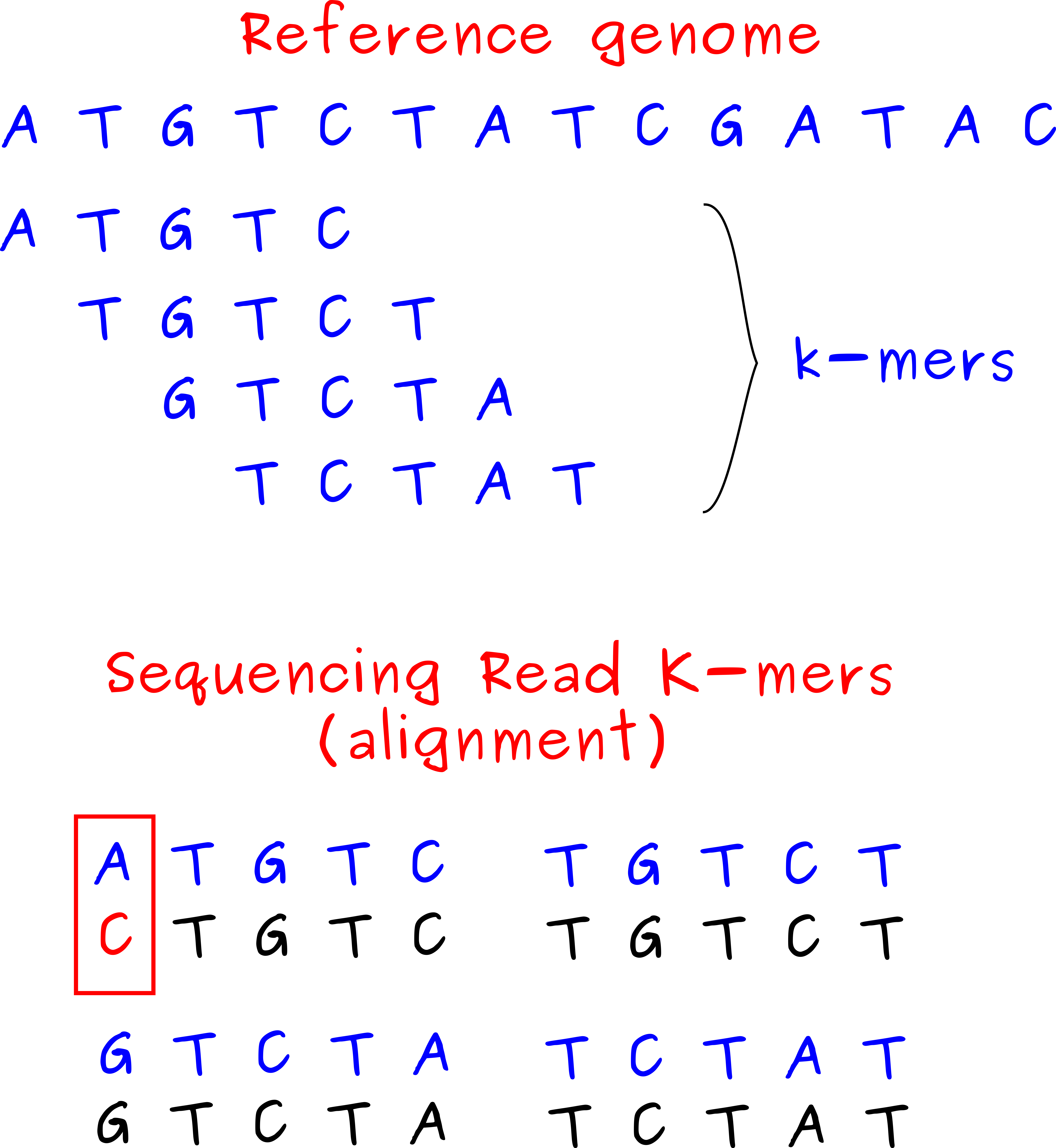
Genome Alignment
The next task is to align our sequenced reads back to the genome. This is done using alignment algorithms but is essentially like piecing a puzzle back together! In the bottom half of the figure a mismatch is highlighted – we know that adenine cannot pair with cytosine. The algorithm will retain this read as the majority of the read aligns to the genome, 4 of 5 bases are a perfect match. Later, we can check if this mismatch is a one-off (likely a sequencing error) or if this error occurs in multiple reads covering the site. This would be indicative of a DNA mutation in the person’s DNA that is different to the healthy reference. This technique of identifying mutations is called variant calling – another popular branch of bioinformatics not covered in this course.

Viewing Alignments
Exercises – Viewing Alignments
This is difficult to conceptualise so let’s get some hands on experience with a file containing aligned reads.
- Navigate to https://igv.org/app/
- In the dropdown menu, select ‘Genome’, > ‘sacCer3’
- Navigate to the following web page: https://github.com/BarryDigby/Youth-Academy/tree/master/data.
- Download the two files
RAP1_UNINDUCED_REP1.markdup.sorted.bamandRAP1_UNINDUCED_REP1.markdup.sorted.bam.bai. - In the dropdown menu, select ‘Tracks’ > ‘Local File’
- Upload the two files you downloaded, they are probably under downloads. Use the shift key to select both files at once.
- To see the reads, you need to zoom in on a gene. Type ‘chrI:87,174-87,813’ into the search bar to view the SCN1 gene.
- The histogram depicts the read coverage at the SCN1 gene. Scroll down in the interactive viewer to see the reads.
Bonus: there is a read with a green A highlighted – this is an example of a mismatch from the reference genome.
3. Data Analysis
Examples of data analysis that can be performed on RNA-Seq data will be provided in worksheets throughout the course.

